Multistage Graph

 Dynamic Programming 

Dynamic Programming is also used in optimization problems.  Like divide-and-conquer method, Dynamic Programming  solves problems by combining the solutions of sub problems.  Moreover, Dynamic Programming algorithm solves each sub 

problem just once and then saves its answer in a table,  thereby avoiding the work of re-computing the answer every  time. 

Two main properties of a problem suggest that the given  problem can be solved using Dynamic Programming. These  properties are overlapping sub-problems and optimal  substructure. 

Steps of Dynamic Programming Approach 

Dynamic Programming algorithm is designed using the  following four steps − 

• Characterize the structure of an optimal solution. • Recursively define the value of an optimal solution. • Compute the value of an optimal solution, typically in a  bottom-up fashion. 

• Construct an optimal solution from the computed  information. 

Applications of Dynamic Programming Approach 

• Matrix Chain Multiplication 

• Longest Common Subsequence 

• Travelling Salesman Problem 

Multistage graph problem 

1. The multistage graph problem is to find a minimum cost  from a source to a sink. 

2. A multistage graph is a directed graph having a number of  multiple stages, where stages element should be  connected consecutively.

3. In this multiple stage graph, there is a vertex whose in  degree is 0 that is known as the source. And the vertex  with only one out degree is 0 is known as the destination  vertex. 

4. The one end of the multiple stage graphs is at i thus the  other reaching end is on i+1 stage. 

5. If we denote a graph G = (V, E) in which the vertices are  partitioned into K >= 2 disjoints sets, Vi, 1 <= I <=K. So  that, if there is an edge < u, v > from u to v in E, the u  £Vi and v € v (i+1), for some I, 1 <= i<= K. And  

sets V1 and Vk are such that |V1| = |Vk| = 1. 

Algorithm for Forward Approach 

1. F graph (graph G, int K, int n,  intp[])   2. {   3. Float cost [max size], int d [max  size], r;   4. Cost [n] = 0.0   5. For (int j = n-1; j>= 1; j--)  6. {   7. Let r be a vertex such that is an  edge of G and C[j][r] + cost[r] is minimum;  8. Cost [j] = C[j][r] + Cost[r]  9. D [j] = r   10. }   11. P [1] = 1 , P[k] = n   12. For (j = 2 ; j <= K-1; j++)  13. P[j] = d[P(j-1)];   14. }

Input = input is a K stage graph G = (V, E) with n vertices  indexed in order of stages. 

E is a set of an edge. 

C [i][j] is the cost or weight of the edge [i][j]

Algorithm for Backward Approach 

1. Algorithm BGraph (G, K, n, p)   2. // some function as FGraph   3. {   4. B cost [1] = 0.0;   5. For j = 2 to n do   6. {   7. // compute b cost [j].   8. Let r be such that is an edge of   9. G and b cost [r] + c [r, j];  10. D [j] = r;   11. }   12. // find a minimum cost path  13. P [1] = 1; p [k] = n;  14. For j = k-1 to 2 do p[j] = d [p  (j+1)];   15. }

If we consider s as the vertex in V1 and t as the vertex in Vk.  The vertex s is supposed as the source and vertex t as the sink.  The cost of a path from s to t is the sum of the costs of the  edges on the path. 

Here, each set Vi defines a stage in the graph. Each path starts  from stage 1 goes to stage 2 then to stage 3 and so on,  because of constraints on E.

The minimum cost of s to t path is indicated by a dashed line.  This method can be used for solving many problems such as  allocating some resources to given number of projects with the  intent to find the maximum profit. 

Consider the graph G as shown in the figure. 

There is a single vertex in stage 1, then 3 vertices in stage 2, then 2  vertices in stage 3 and only one vertex in stage 4 (this is a target  stage). 

Backward approach 

d(S, T)=min {1+d(A, T),2+d(B,T),7+d(C,T)} …(1)

We will compute d(A,T), d(B,T) and d(C,T). d(A,T)=min{3+d(D,T),6+d(E,T)} …(2) d(B,T)=min{4+d(D,T),10+d(E,T)} …(3) d(C,T)=min{3+d(E,T),d(C,T)} …(4) 

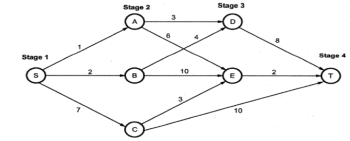
Now let us compute d(D,T) and d(E,T). d(D,T)=8 

d(E,T)=2 backward vertex=E 

Let us put these values in equations (2), (3) and (4) d(A,T)=min{3+8, 6+2} 

d(A,T)=8 A-E-T 

d(B,T)=min{4+8,10+2} 

d{B,T}=12 A-D-T 

d(C,T)=min(3+2,10) 

d(C,T)=5 C-E-T 

d(S,T)=min{1+d(A,T), 2+d(B,T), 7+d(C,T)} =min{1+8, 2+12,7+5} 

=min{9,14,12}

d(S,T)=9 S-A-E-T 

The path with minimum cost is S-A-E-T with the cost 9. Forward approach 

d(S,A)=1 

d(S,B)=2 

d(S,C)=7 

d(S,D)=min{1+d(A,D),2+d(B,D)} 

=min{1+3,2+4} 

d(S,D)=4 

d(S,E)=min{1+d(A,E), 2+d(B,E),7+d(C,E)} =min {1+6,2+10,7+3} 

=min {7,12,10} 

d(S,E)=7 i.e. Path S-A-E is chosen. 

d(S,T)=min{d(S,D)+d(D,T),d(S,E),d(E,T),d(S,C)+d(C,T)} =min {4+8,7+2,7+10} 

d(S,T)=9 i.e. Path S-E, E-T is chosen. 

The minimum cost=9 with the path S-A-E-T.

Using dynamic approach programming strategy, the  multistage graph problem is solved. This is because in  multistage graph problem we obtain the minimum path at  each current stage by considering the path length of each  vertex obtained in earlier stage. 

Thus the sequence of decisions is taken by considering overlapping solutions. In  dynamic programming, we may get any number of solutions for given problem.  From all these solutions we seek for optimal solution, finally solution becomes  the solution to given problem. Multistage graph problem is solved using this  same approach. 

4 

A D 

1 

11 

5 

9 

18 

2 13 B E 

S T 

5 

Backward approach 

16 

2

C F 2 

d(S,T) = min{1+d(A,T), 2+d(B,T),5+d(C,T)---------1 d(A,T) = min {4+d(D,T), 11+d(E,T) 

=min{4+18,11+13} 

=min{22,24} 

=22 

d(B,T) = min{9+d(D,T),5+d(E,T),16+d(F,T) =min{9+18,5+13,16+2} 

=min(27,18,18} 

=18 

D(C,T)=2+2 

= 4 

d(S,T) = min{1+d(A,T), 2+d(B,T),5+d(C,T)---------1 =min{1+22,2+18,5+4} 

=min(23,20,9} 

=9 S-C-F-T 

Forward approach 

d(S,A)=1 

d(S,B)=2 

d(S,C)=5 

d(S,D)=min{1+d(A,D),2+d(B.D)} 

1 

4 

A D 

18 

= min{1+4,2+9}  =min{5,11} 

11 

5 

9 

2 13 B E 

S T 

=5 

D(S,E) = min{1+d(A,E),2+d(B,E)} 

5 

= {1+11,2+5} 

={12.7} 

=7 

D(S,F)=min{2+d(B,F),5+d(C,F)} 

 =min{2+16,5+2} 

Min{18,7} 

=7 

16 

2

C F 2 

D(S,T) =min{d(S,D)+d(D,T),d(S,E)+d(E,T),d(S,F)+d(F,T)} =min {5+18,7+13,7+2} 

= min{23,20,9} 

=9 

Example3: 

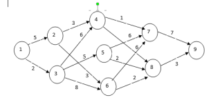
Backward approach 

d(1,9)= min{5+d(2,9),2+d(3,9)} --------1 

d(2,9)= min{3+d(4,9), 3+d(6,9)}--------2 d(4,9)= min{1+d(7,9), 4+d(8,9)} 

 =min{1+7,4+3} 

 =min(8,7} 

 =7 

d(6,9) =min { 6+d(7,9), 2+d(8,9)} 

 =min{6+7,2+3} 

=min{ 13,5} 

=5 

d(2,9)= min{3+d(4,9), 3+d(6,9)}--------2 =min {3+7. 3+5} 

=min{10,8} 

=8

d(3,9)= min{6+d(4,9), 5+d(5,9),8+d(6,9)} 

d(4,9) = 7 

d(5,9) = min{6+d(7,9), 2+d(8,9)} 

=min{6+7, 2+3} 

=min{13,5} 

= 5 

d(6,9) =5 

d(3,9)= min{6+d(4,9), 5+d(5,9),8+d(6,9)} 

=min {6+7,5+5,8+5} 

=min{13,10,13} 

=10 

d(1,9)= min{5+d(2,9),2+d(3,9)} --------1 

=min{5+8,2+10} 

=min{13,12} 

=12 

Path is 1 3 5 8 9

Forward approach 

d(1,2) = 5 

d(1,3) = 2 

d(1,4)= min{5+d(2,4),2+d(3,4) } 

=min(5+3, 2+6} = min {8,8} = 8 

d(1,5)= 2+d(3,5) = 2+5 = 7 

d(1,6) = min{5+d(2,6), 2+d(3,6) 

=min{ 5+3, 2+8} = min{8,10} =8 

d(1,7)= min{d(1,4)+d(4,7), d(1,5)+d(5,7), d(1,6)+d(6,7)} = min{8+1,7+ 6, 8+6} 

=min {9,13,14}  

= 9 

d(1,8)= min{ d(1,4)+d(4,8), d(1,5) +d(5,8), d(1,6)+ d(6,8)} ={13,9,10} 

=9 

d(1,9) = min{d(1,7)+d(7,9) , d(1,8) +d(8,9)} 

 = min(9+7,9+3} 

=12

Example :4 Solve using Forward & Backword Approach 

Example 5: Solve using Forward & Backword Approach