Computer Graphics : 01
1.0 Objectives
At the end of this chapter the reader will be able to:
• Describe Computer Graphics and its applications.
• Describe and distinguish between Interactive and Passive Graphics. • Describe advantages of Interactive Graphics.
• Describe applications of Computer Graphics.
Structure
1.1 Introduction
1.2 Interactive Graphics
1.3 Passive Graphics
1.4 Advantages of Interactive Graphics
1.5 How the Interactive Graphics Display Works
1.6 Applications of Computer Graphics
1.7 Summary
1.8 Keywords
1.9 Self Assessment Questions (SAQ)
1.10 References/Suggested Readings
1.1 Introduction
The term computer graphics includes almost everything on computers that is not text or sound. Today almost every computer can do some graphics, and people have even come to expect to control their computer through icons and pictures rather than just by typing. Here in our lab at the Program of Computer Graphics, we think of computer graphics as drawing pictures on computers, also called rendering. The pictures can be photographs, drawings, movies, or simulations - pictures of things, which do not yet exist and maybe could never exist. Or they may be pictures from places we cannot see directly, such as medical images from inside your body. We spend much of our time improving the way computer pictures can simulate real world scenes. We want images on computers to not just look more realistic, but also to be more realistic in their colors, the way objects and rooms are lighted, and the way different materials appear. We call this work “realistic image synthesis”.
1.2 Interactive Graphics
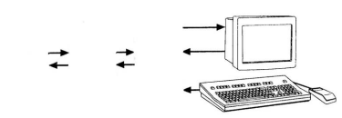
In interactive computer graphics user have some control over the picture i.e user can make any change in the produced image. One example of it is the ping pong game. The conceptual model of any interactive graphics system is given in the picture shown in Figure 1.1. At the hardware level (not shown in picture), a computer receives input from interaction devices, and outputs images to a display device. The software has three components. The first is the application program, it creates, stores into, and retrieves from the second component, the application model, which represents the the graphic primitive to be shown on the screen. The application program also handles user input. It produces views by sending to the third component, the graphics system, a series of graphics output commands that contain both a detailed geometric description of what is to be viewed and the attributes describing how the objects should appear. After the user input is processed, it sent to the graphics system is for actually producing the picture. Thus the graphics system is a layer in between the application program and the display hardware that effects an output transformation from objects in the application model to a view of the model.
Applicatio Applicati n Program on Model
Graphics system
Figure 1.1: Conceptual model for interactive graphics
The objective of the application model is to captures all the data, objects, and relationships among them that are relevant to the display and interaction part of the application program and to any nongraphical postprocessing modules.
1.3 Passive Graphics
A computer graphics operation that transfers automatically and without operator intervention. Non-interactive computer graphics involves one way communication between the computer and the user. Picture is produced on the monitor and the user does not have any control over the produced picture.
1.4 Advantages of Interactive Graphics
Graphics provides one of the most natural means of communicating with a computer, since our highly developed 2D and 3D pattern-recognition abilities allow us to perceive and process pictorial data rapidly and efficiently. In Many design, implementation, and construction processes today, the information pictures can give is virtually indispensable. Scientific visualization became an important field in the late 1980s, when scientists and engineers realized that they could not interpret the data and prodigious quantities of data produced in supercomputer runs without summarizing the data and highlighting trends and phenomena in various kinds of graphical representations.
Creating and reproducing pictures, however, presented technical problems that stood in the way of their widespread use. Thus, the ancient Chinese proverb “a picture is worth
ten thousand words” became a cliché in our society only after the advent of inexpensive and simple technology for producing pictures—first the printing press, then photography.
Interactive computer graphics is the most important means of producing pictures since the invention of photography and television; it has the added advantage that, with the computer, we can make pictures not only of concrete, “real-world” objects but also of abstract, synthetic objects, such as mathematical surfaces in 4D and of data that have no inherent geometry, such as survey results. Furthermore, we are not confined to static images. Although static pictures are a good means of communicating information, dynamically varying pictures are frequently even better–to time-varying phenomena, both real (e.g., growth trends, such as nuclear energy use in the United States or population movement form cities to suburbs and back to the cities). Thus, a movie can show changes over time more graphically than can a sequence of slides. Thus, a sequence of frames displayed on a screen at more than 15 frames per second can convey smooth motion or changing form better than can a jerky sequence, with several seconds between individual frames. The use of dynamics is especially effective when the user can control the animation by adjusting the speed, the portion of the total scene in view, the amount of detail shown, the geometric relationship of the objects in the another, and so on. Much of interactive graphics technology therefore contains hardware and software for user controlled motion dynamics and update dynamics.
With motion dynamics, objects can be moved and tumbled with respect to a stationary observer. The objects can also remain stationary and the viewer can move around them , pan to select the portion in view, and zoom in or out for more or less detail, as though looking through the viewfinder of a rapidly moving video camera. In many cases, both the objects and the camera are moving. A typical example is the flight simulator, which combines a mechanical platform supporting a mock cockpit with display screens for windows. Computers control platform motion, gauges, and the simulated world of both stationary and moving objects through which the pilot navigates. These multimillion dollar systems train pilots by letting the pilots maneuver a simulated craft over a simulated 3D landscape and around simulated vehicles. Much simpler fight simulators are among the most popular games on personal computers and workstations. Amusement
parks also offer “motion-simulator” rides through simulated terrestrial and extraterrestrial landscapes. Video arcades offer graphics-based dexterity games and racecar-driving simulators, video games exploiting interactive motion dynamics: The player can change speed and direction with the “gas pedal” and “steering wheel,” as trees, buildings, and other cars go whizzing by. Similarly, motion dynamics lets the user fly around the through buildings, molecules, and 3D or 4D mathematical space. In another type of motion dynamics, the “camera” is held fixed, and the objects in the scene are moved relative to it. For example, a complex mechanical linkage, such as the linkage on a stream engine, can be animated by moving or rotating all the pieces appropriately.
Update dynamics is the actual change of the shape, color, or other properties of the objects being viewed. For instance, a system can display the deformations of an airplane structure in flight or the state changes in a block diagram of a nuclear reactor in response to the operator’s manipulation of graphical representations of the many control mechanisms. The smoother the change, the more realistic and meaningful the result. Dynamic interactive graphics offers a large number of user-controllable modes with which to encode and communicate information: the 2D or 3D shape of objects in a picture, their gray scale or color, and the time variations of these properties. With the recent development of digital signal processing (DSP) and audio synthesis chips, audio feedback can now be provided to augment the graphical feedback and to make the simulated environment even more realistic.
Interactive computer graphics thus permits extensive, high-bandwidth user-computer interaction. This significantly enhances our ability to understand data, to perceive trends, and to visualize real or imaginary objects–indeed, to create “virtual worlds” that we can explore from arbitrary points of view. By making communication more efficient, graphics make possible higher-quality and more precise results or products, greater productivity, and lower analysis and design costs.
1.5 How The Interactive Graphics Display Works
The modern graphic display is very simple in construction. It consists of the three components shown in figure 1.2 below.
(1) Frame Buffer
(2) Monitor like a TV set without the tuning and receiving electronics. (3) Display Controller It passes the contents of the frame buffer to the monitor.
00000000 00000001 00000000 00011001
Scan Line Data
Scan Line
01111100 01100001
00110000 00011101
11100000 00001001
………… …………
00000000 11000001 00001110 01110001 00000000 00011101 00001110 00001001 00000000 00001001 00011110 00010001 00000000 00110001 00000000 10000001 00011110 11000001 00000001 00110001 00000110 10000001
Display Controller Figure 1.2
…………………………. ………………………… .
.
.
.
.
.
………………………….
Inside the frame buffer the image is stored as a pattern of binary digital numbers, which represent a array of picture elements, or pixels. In the simplest case, where you want to store only black and white images, you can represent black pixels by “1’s” and white pixels by “0’s” in the frame buffer. Therefore, a array of black and white pixels of 16X16 could be represented by 32 bytes, stored in frame buffer.
The display controller reads each successive byte of data from the frame buffer and converts its 0’s and 1’s into corresponding video signals. This signal is then fed to the monitor, producing a black and white image on the screen. The display controller repeats this operation 30 times a second to maintain a steady picture on the monitor. If you want to change the image, then you need to modify the frame buffer’s contexts to represent the new pattern of pixels.
1.6 Applications of Computer Graphics
Classification of Applications
The diverse uses of computer graphics listed in the previous section differ in a variety of ways, and a number of classification is by type (dimensionality) of the object to be represented and the kind of picture to be produced. The range of possible combinations is indicated in Table 1.1.
Table 1.1
Computer graphics is used today in many different areas of industry, business, government, education, entertainment, and most recently, the home. The list of applications is enormous and is growing rapidly as computers with graphics capabilities become commodity products. Let`s look at a representative sample of these areas.
Cartography: Computer graphics is used to produce both accurate and schematic representations of geographical and other natural phenomena from measurement data. Examples include geographic maps, relief maps, exploration maps for drilling and mining, oceanographic charts, weather maps, contour maps, and population
density maps.
User interfaces: As soon mentioned, most applications that run on personal computers and workstations, and even those that run on terminals attached to time shared computers and network compute servers, have user interfaces that rely on desktop window systems to manage multiple simultaneous activities, and on point and click facilities to allow users to select menu items, icons, and objects on the screen; typing is necessary only to input text to be stored and manipulated. Word
processing , spreadsheet, and desktop-publishing programs are typical applications that take
Advantage of such user-interface techniques: The authors of this book used such programs to create both the text and the figures; then , the publisher and their contractors produced the book using similar typesetting and drawing software.
(Interactive) plotting in business, science and technology: The next most common use of graphics today is probably to create 2D and 3D graphs of mathematical, physical, and economic functions; histograms, bar and pie charts; task-scheduling charts; inventory and production charts, and the like . All these are used to present meaningfully and concisely the trends and patterns gleaned from data, so as to clarify complex phenomena and to facilitate informed decision making.
Office automation and electronic publishing: The use of graphics for the creation and dissemination of information has increased enormously since the advent of desktop publishing on personal computers. Many organizations whose publications used to be printed by outside specialists can now produce printed materials inhouse. Office automation and electronic publishing can produce both traditional printed (hardcopy) documents and electronic (softcopy) documents that allow browsing of networks of interlinked multimedia documents are proliferating
Computer-aided drafting and design: In computer-aided design (CAD), interactive graphics is used to design components and systems of mechanical , electrical, electromechanical, and electronic devices, including structure such as buildings, automobile bodies, airplane and ship hulls, very large scale-integrated (VLSI) chips, optical systems, and telephone and computer networks. Sometimes, the use; merely wants to produce the precise drawings of components and assemblies, as for online
drafting or architectural blueprints Color Plate 1.8 shows an example of such a 3D design program, intended for nonprofessionals also a customize your own patio deck” program used in lumber yards. More frequently however the emphasis is on interacting with a computer based model of the component or system being designed in order to test, for example, its structural, electrical, or thermal properties. Often, the model is interpreted by a simulator that feeds back the behavior of the system to the user for further interactive design and test cycles. After objects have been designed, utility programs can postprocess the design database to make parts lists, to process ‘bills of materials’, to define numerical control tapes for cutting or drilling parts, and so on.
Simulation and animation for scientific visualization and entertainment: Computer produced animated movies and displays or the time-varying behavior of real and simulated objects are becoming increasingly popular for scientific and engineering visualization. We can use them to study abstract mathematical entries as well as mathematical models of such phenomena as fluid flow, relativity, nuclear and chemical reactions, physiological system and organ function, and deformation of mechanical structures under various kinds of loads. Another advanced-technology area is interactive cartooning. The simpler kinds of systems for producing ‘Flat” cartons are becoming cost-effective in creating routine ‘in-between” frames that interpolate between two explicity specified ‘key frames”. Cartoon characters will increasingly be modeled in the computer as 3D shape descriptions whose movements are controlled by computer commands, rather than by the figures being drawn manually by cartoonists . Television commercials featuring flying logos and more exotic visual trickery have become common, as have elegant special effects in movies. Sophisticated mechanisms are available to model the objects and to represent light and shadows.
Art and commerce: Overlapping the previous categories the use of computer graphics in art and advertising here, computer graphics is used to produce pictures that express a message and attract attention. Personal computers and Teletext and Videotexts terminals in public places such as in private homes, offer much simpler
but still informative pictures that let users orient themselves, make choices, or even “teleshop” and conduct other business transactions. Finally, slide production for commercial, scientific, or educational presentations is another cost-effective use of graphics, given the steeply rising labor costs of the traditional means of creating such material.
Process control: Whereas flight simulators or arcade games let users interact with a simulation of a real or artificial world, many other applications enable people or interact with some aspect of the real world itself. Status displays in refineries, power plants, and computer networks show data values from sensors attached to critical system components, so that operators can respond to problematic conditions. For example, military commanders view field data – number and position of vehicles, weapons launched, troop movements, causalities – on command and control displays to revise their tactics as needed; flight controller airports see computer-generated identification and status information for the aircraft blips on their radar scopes, and can thus control traffic more quickly and accurately than they could with the uninitiated radar data alone; spacecraft controllers monitor telemetry data and take corrective action as needed.
1.7 Summary
⌘ Computer graphics includes the process and outcomes associated with using computer technology to convert created or collected data into visual representations.
⌘ Graphical interfaces have replaced textual interfaces as the standard means for user-computer interaction. Graphics has also become a key technology for communicating ideas, data, and trends in most areas of commerce, science, engineering, and education With graphics, we can create artificial realities, each a computer-based “exploratorium” for examining objects and phenomena in a natural and intuitive way that exploits our highly developed skills in visual
pattern recognition.
⌘ Until the late eighties, the bulk of computer-graphics applications dealt with 2D objects, 3D applications were relatively rare, both because 3D software is intrinsically far more complex than is 2D software and because a great deal of computing power is required to render pseudorealistic images. Therefore, until recently, real-time user interaction with 3D models and pseudorealistic images was feasible on only very expensive high-performance workstations with dedicated, special-purpose graphics hardware. The spectacular progress of VLSI semiconductor technology that was responsible for the advent of inexpensive microprocessors and memory led in the early 1980s to the creation of 2D, bitmap-graphics-based personal computers. That same technology has made it possible, less than a decade later, to create subsystems of only a few chips that do real-time 3D animation with color-shaded images of complex objects, typically described by thousands of polygons. These subsystems can be added as 3D accelerators to workstations or even to personal computers using commodity microprocessors It is clear that an explosive growth of 3D applications will parallel the current growth in applications.
⌘ Much of the task of creating effective graphic communication, whether 2D or 3D, lies in modeling the objects whose images we want to produce. The graphics system acts as the intermediary between the application model and the output device. The application program is responsible for creating and updating the model based on user interaction; the graphics system does the best-understood, most routine part of the job when it creates views of objects and passes user events to the application.
1.8 Keywords
Computer Graphics, Interactive Graphics, Passive Graphics
1.9 Self Assessment Questions (SAQ)
1. Write a short note on the interactive computer graphics.
2. Discuss the relative advantage of interactive and passive graphics.
3. What are the applications of computer graphics?
4. Nominate an application of computers that can be accommodated by either textual or graphical computer output. Explain when and why graphics output would be more appropriate in this application.
5. Explain briefly the classification of computer graphics.
1.10 References/Suggested Readings
1. Computer Graphics, Principles and Practice, Second Edition, by James D. Foley, Andries van Dam, Steven K. Feiner, John F. Hughes, Addison- Wesley 2. Computer Graphics , Second Edition , by Pradeep K. Bhatia , I.K .International Publisher.
3. High Resolution Computer Graphics using Pascal/C, by Ian O. Angell and Gareth Griffith, John Wiley & Sons
4. Computer Graphics (C Version), Donald Hearn and M. Pauline Baker, Prentice Hall,
5. Advanced Animation and Rendering Techniques, Theory and Practice, Alan Watt and Mark Watt , ACM Press/Addison-Wesley
6. Graphics Gems I-V, various authors, Academic Press
7. Computer Graphics, Plastok, TMH
8. Principles of Interactive Computer Graphics, Newman, TMH
Author: Abhishek Taneja Vetter: Dr. Pradeep Bhatia Lesson: Display Devices Lesson No. : 02
1.0 Objectives
At the end of this chapter the reader will be able to:
• Describe and distinguish raster and random scan displays
• Describe various display devices.
• Describe how colour CRT works..
Structure
2.1 Introduction
2.2 Refresh CRT
2.3 Random-Scan and Raster Scan Monitor
2.4 Color CRT Monitors
2.5 Direct-View Storage Tubes (DVST)
2.6 Flat-Panel Displays
2.7 Light-emitting Diode (LED) and Liquid-crystal Displays (LCDs) 2.8 Hard Copy Devices
2.9 Summary
2.10 Key Words
2.11 Self Assessment Questions (SAQ)
2.12 References/Suggested Readings
2.1 Introduction
The principle of producing images as collections of discrete points set to appropriate colours is now widespread throughout all fields of image production. The most common graphics output device is the video monitor which is based on the standard cathode ray tube(CRT) design, but several other technologies exist and solid state monitors may eventually predominate.
2.2 Refresh CRT
Basic Operation of CRT
Figure 2.1 illustrates the basic operation of a CRT. A beam of electrons (cathode rays), emitted by an electron gun, passes through focusing and deflection systems that direct the beam toward specified positions on the phosphor-coated screen.
Figure 2.1: Basic Design of a magnetic-deflection CRT

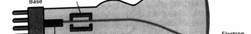
The phosphor then emits a small spot of light at each position contacted by the electron beam. Because the light emitted by the phosphor fades very rapidly, some method is needed for maintaining the screen picture. One Way to keep the phosphor glowing is to redraw the picture repeatedly by quickly directing the electron beam back over the same points. This type of display is called a refresh CRT.
Working
Beam passes between two pairs of metal plates, one vertical and other horizontal. A voltage difference is applied to each pair of plates according to the amount that the beam
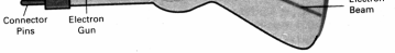
is to be deflected in each direction. As the electron beam passes between each pair of plates, it is bent towards the plate with the higher positive voltage. In figure 2.2 the beam is first deflected towards one side of the screen. Then, as the beam passes through the horizontal plates, it is deflected towards, the top or bottom of the screen. To get the proper deflection, adjust the current through coils placed around the outside of the CRT loop. The primary components of an electron gun in a CRT are the heated metal cathode and a control grid (Fig. 2.2). Heat is supplied to the cathode by directing a current through a coil of wire, called the filament, inside the cylindrical cathode structure. This causes electrons to be "boiled off" the hot cathode surface. In the vacuum inside the CRT envelope, the free, negatively charged electrons are then accelerated toward the phosphor coating by a high positive voltage. The accelerating voltage can be generated with a positively charged metal coating on the in- side of the CRT envelope near the phosphor screen, or an accelerating anode can be used, as in Fig. 2.2. Sometimes the electron gun is built to contain the accelerating anode and focusing system within the same unit.
Figure 2.2: Operation of an electron gun with an acceleration anode
The focusing system in a CRT is needed to force the electron beam to converge into a small spot as it strikes the phosphor. Otherwise, the electrons would repel each other, and the beam would spread out as it approaches the screen. Focusing is accomplished with either electric or magnetic fields. Electrostatic focusing is commonly used in television and computer graphics monitors. With electrostatic focusing, the electron beam passes through a positively charged metal cylinder that forms an electrostatic lens, as shown in Fig. 2.3. The action of the electrostatic lens focuses the electron beam at the center of the
screen, in exactly the same way that an optical lens focuses a beam of light at a particular focal distance. Similar lens focusing effects can be accomplished with a magnetic field set up by a coil mounted around the outside of the CRT envelope. Magnetic lens focusing produces the smallest spot size on the screen and is used in special-purpose devices.
As with focusing, deflection of the electron beam can be controlled either with electric fields or with magnetic fields. Cathode-ray tubes are now commonly constructed with magnetic deflection coils mounted on the outside of the CRT envelope, as illustrated in Fig. 2.1. Two pairs of coils are used, with the coils in each pair mounted on opposite sides of the neck of the CRT envelope. One pair is mounted on the top and bottom of the neck, and the other pair is mounted on opposite sides of the neck. The magnetic field produced by each pair of coils results in a transverse deflection force that is perpendicular both to the direction of the magnetic field and to the direction of travel of the electron beam. Horizontal deflection is accomplished with one pair of coils, and vertical deflection by the other pair. The proper deflection amounts are attained by adjusting the current through the coils. When electrostatic deflection is used, two pairs of parallel plates are mounted inside the CRT envelope. One pair of plates is mounted horizontally to control the vertical deflection, and the other pair is mounted vertically to control horizontal deflection (Fig. 2.3).
Figure 2.3: Electrostatic deflection of the electron beam in a CRT


Spots of light are produced on the screen by the transfer of the CRT beam energy to the phosphor. When the electrons in the beam collide with the phosphor coating, they are stopped and their kinetic energy is absorbed by the phophor. Part of the beam energy is converted by friction into heat energy, and the remainder causes electrons in the phosphor
atoms to move up to higher quanturn-energy levels. After a short time, the "excited" phosphor electrons begin dropping back to their stable ground state, giving up their extra energy as small quantums of light energy. What we see on the screen is the combined effect of all the electron light emissions: a glowing spot that quickly fades after all the excited phosphor electrons have returned to their ground energy level. The frequency (or color) of the light emitted by the phosphor is proportional to the energy difference between the excited quantum state and the ground state.
Figure 2.4 shows the intensity distribution of a spot on the screen. The intensity is greatest at the center of the spot, and decreases with a Gaussian distribution out to the edges of the spot. This distribution corresponds to the cross-sectional electron density distribution of the CRT beam.

Figure 2.4: Intensity distribution of an illuminated phosphor spot on a CRT screen Resolution
The maximum number of points that can be displayed without overlap on a CRT is referred to as the resolution. A more precise definition of resolution is the number of points per centimeter that can be plotted horizontally and vertically, although it is often simply stated as the total number of points in each direction. This depends on the type of phosphor used and the focusing and deflection system.
Aspect Ratio
Another property of video monitors is aspect ratio. This number gives the ratio of vertical points to horizontal points necessary to produce equal-length lines in both directions on the screen. (Sometimes aspect ratio is stated in terms of the ratio of horizontal to vertical points.) An aspect ratio of 3/4 means that a vertical line plotted with three points has the same length as a horizontal line plotted with four points.
2.3 Random-Scan and Raster Scan Monitor
2.3.1 Random-Scan/Calligraphic displays
Random scan system uses an electron beam which operates like a pencil to create a line image on the CRT. The image is constructed out of a sequence of straight line segments. Each line segment is drawn on the screen by directing the beam to move from one point on screen to the next, where each point is defined by its x and y coordinates. After drawing the picture, the system cycles back to the first line and design all the lines of the picture 30 to 60 time each second. When operated as a random-scan display unit, a CRT has the electron beam directed only to the parts of the screen where a picture is to be drawn. Random-scan monitors draw a picture one line at a time and for this reason are also referred to as vector displays (or stroke-writing or calligraphic displays) Fig. 2.5. A pen plotter operates in a similar way and is an example of a random-scan, hard-copy device.


Figure 2.5: A random-scan system draws the component lines of an object in any order specified
Refresh rate on a random-scan system depends on the number of lines to be displayed. Picture definition is now stored as a set of line-drawing commands in an area of memory referred to as the refresh display file. Random-scan systems are designed for line-drawing
applications and can-not display realistic shaded scenes. Since picture definition is stored as a set of line-drawing instructions and not as a set of intensity values for all screen points, vector displays generally have higher resolution than raster systems. Also, vector displays produce smooth line drawings because the CRT beam directly follows the line path.
2.3.2 Raster-Scan Displays
In raster scan approach, the viewing screen is divided into a large number of discrete phosphor picture elements, called pixels. The matrix of pixels constitutes the raster. The number of separate pixels in the raster display might typically range from 256X256 to 1024X 1024. Each pixel on the screen can be made to glow with a different brightness. Colour screen provide for the pixels to have different colours as well as brightness. In a raster-scan system, the electron beam is swept across the screen, one row at a time from top to bottom. As the electron beam moves across each row, the beam intensity is turned on and off to create a pattern of illuminated spots. Picture definition is stored in a memory area called the refresh buffer or frame buffer. This memory area holds the set of intensity values for all the screen points. Stored intensity values are then retrieved from the refresh buffer and "painted" on the screen one row (scan line) at a time (Fig. 2.6). Each screen point is referred to as a pixel or pel (shortened forms of picture element). The capability of a raster-scan system to store intensity information for each screen point makes it well suited for the realistic display of scenes containing subtle shading and color patterns. Home television sets and printers are examples of other systems using raster scan methods.
Figure 2.6: A raster-scan system displays an object as a set of discrete points across each scan line
Intensity range for pixel positions depends on the capability of the raster system. In a simple black-and-white system, each screen point is either on or off, so only one bit per pixel is needed to control the intensity of screen positions. For a bilevel system, a bit value of 1 indicates that the electron beam is to be turned on at that position, and a value of 0 indicates that the beam intensity is to be off. Additional bits are needed when color and intensity variations can be displayed. On some raster-scan systems (and in TV sets), each frame is displayed in two passes using an interlaced refresh procedure. In the first pass, the beam sweeps across every other scan line from top to bottom. Then after the vertical re- trace, the beam sweeps out the remaining scan lines (Fig. 2.7). Interlacing of the scan lines in this way allows us to see the entire screen displayed in one-half the time it would have taken to sweep across all the lines at once from top to bottom. Interlacing is primarily used with slower refreshing rates. On an older, 30 frame- per-second, noninterlaced display, for instance, some flicker is noticeable. But with interlacing, each of the two passes can be accomplished in l/60th of a second, which brings the refresh rate nearer to 60 frames per second. This is an effective technique for avoiding flicker, providing that adjacent scan lines contain similar display information.
Figure 2.7: Interlacing Scan lines on a raster-scan display. First , all points on the even-numbered (solid) scan lines are displayed; then all points along the odd numbered (dashed) lines are displayed
2.4 Color CRT Monitors
To display colour pictures, combination of phosphorus is used that emits different coloured light. There are two different techniques for producing colour displays with a CRT.
1. Beam Penetration Method
2. Shadow Mask Method
Beam Penetration Method
The beam-penetration method for displaying color pictures has been used with random scan monitors. Two layers of phosphor, usually red and green, are coated onto the inside of the CRT screen, and the displayed color depends on how far the electron beam penetrates into the phosphor layers. A beam of slow electrons excites only the outer red layer. A beam of very fast electrons penetrates through the red layer and excites the inner green layer. At intermediate beam speeds, combinations of red and green light are emitted to show two additional colors, orange and yellow. The speed of the electrons, and hence the screen color at any point, is controlled by the beam-acceleration voltage. Beam penetration has been an inexpensive way to produce color in random-scan monitors, but only four colors are possible, and the quality of pictures is not as good as with other methods.
Shadow Mask Method
Shadow-mask methods are commonly used in raster-scan systems (including color TV) because they produce a much wider range of colors than the beam-penetration method. A shadow-mask CRT has three phosphor color dots at each pixel position. One phosphor dot emits a red light, another emits a green light, and the third emits a blue light. This type of CRT has three electron guns, one for each color dot, and a shadow-mask grid just behind the phosphor-coated screen. Figure 2.8 illustrates the delta-delta shadow-mask method, commonly used in color CRT- systems. The three electron beams are deflected and focused as a group onto the shadow mask, which contains a series of holes aligned with the phosphor-dot patterns. When the three beams pass through a hole 'in the shadow mask, they activate a dot triangle, which appears as a small color spot on the screen. The phosphor dots in the triangles are arranged so that each electron beam can activate only its corresponding color dot when it passes through the shadow mask. Another configuration for the three electron guns is an in-line arrangement in which the three electron guns, and the. Corresponding red-green-blue color dots on the screen, are aligned along one scan line instead of in a triangular pattern. This in-line arrangement of electron guns is easier to keep in alignment and is commonly used in high-resolution color CRTs.
Figure 2.8: Operation of a delta–delta, shadow-mask CRT. Three electron guns, aligned with the triangular color-dot patterns on the screen, are directed to each dot triangle by a shadow mask.
We obtain color variations in a shadow-mask CRT by varying the intensity levels of the three electron beams. By turning off the red and green guns, we get only the color coming from the blue phosphor. Other combinations of beam intensities produce a small light spot for each pixel position, since our eyes tend to merge the three colors into one composite. The color we see depends on the amount of excitation of the red, green, and blue phosphors. A white (or gray) area is the result of activating all three dots with equal intensity. Yellow is produced with the green and red dots only, magenta is produced with the blue and red dots, and cyan shows up when blue and green are activated equally. In some low-cost systems, the electron beam can only be set to on or off, limiting displays to eight colors. More sophisticated systems can set intermediate intensity levels for the electron beams, allowing several million different colors to be generated.
2.5 Direct-View Storage Tubes (DVST)
This is an alternative method to monitor a screen image, as it sores the picture information inside the CRT instead of refreshing the screen. A direct-view storage tube (DVST) stores the picture information as a charge distribution just behind the phosphor coated screen. Two electron guns are used in a DVST. One, the primary gun, is used to store the picture pattern; the second, the flood gun, maintains the picture display. A DVST monitor has both disadvantages and advantages compared to the refresh CRT. Because no refreshing is needed, very complex pictures can be displayed at very high resolutions without flicker. Disadvantages of DVST systems are that they ordinarily do not display color and that selected parts of a picture cannot be erased. To eliminate a picture section, the entire screen must be erased and the modified picture redrawn. The erasing and redrawing process can take several seconds for a complex picture. For these reasons, storage displays have been largely replaced by raster systems.
2.6 Flat-Panel Displays
The term flat panel display refers to a class of video device that have reduced volume , weight and power requirement compared to a CRT. A significant feature of flat-panel displays is that they are thinner than CRTs, and we can hang them on walls or wear them on our wrists. Since we can even write on some flat-panel displays, they will soon be available as pocket notepads. Current uses for flat-panel displays include small TV monitors, calculators, pocket video games, laptop computers, armrest viewing of movies on airlines, as advertisement boards in elevators, and as graphics displays in applications requiring rugged, portable monitors.
We can separate flat-panel displays into two categories: emissive displays and nonemissive displays. The emissive displays (or emitters) are devices that convert electrical energy into light. Plasma panels, thin-film electroluminescent displays, and light-emitting diodes are examples of emissive displays. Flat CRTs have also been devised, in which electron beams are accelerated parallel to the screen, then deflected 90° to the screen. But flat CRTs have not proved to be as successful as other emissive devices. Nonemmissive displays (or nonemitters) use optical effects to convert sunlight or light from some other source into graphics patterns. The most important example of a nonemissive flat-panel display is a liquid-crystal device.
2.7 Light-emitting Diode (LED) and Liquid-crystal Displays (LCDs) 2.7.1 Light-emitting Diode (LED)
In LED, a matrix of diodes is arranged to form the pixel positions in the display and picture definition is stored in a refresh buffer. Information is read from the refresh buffer and converted to voltage levels that are applied to the diodes to produce the light patterns in the display.
2.7.2 Liquid-crystal Displays (LCDs)
Liquid crystal displays are the divices that produce a picture by passing polarized light from the surroundings or from an internal light source through a liquid crystal material that transmit the light. Liquid-crystal displays (LCDs) are commonly used in small systems, such ' as calculators and portable, laptop computers. These non-emissive devices produce a picture by passing polarized light from the surroundings or from an internal
light source through a liquid-crystal material that can be aligned to either block or transmit the light.
The term liquid crystal refers to the fact that these compounds have a crystalline arrangement of molecules, yet they flow like a liquid. Flat-panel displays commonly use nematic (threadlike) liquid-crystal compounds that tend to keep the long axes of the rod shaped molecules aligned. A flat-panel display can then be constructed with a nematic liquid crystal, as demonstrated in Fig. 2-9. Two glass plates, each containing a light polarizer at right angles to the other plate, sandwich the liquid-crystal material. Rows of horizontal transparent conductors are built into one glass plate, and columns of vertical conductors are put into the other plate. The intersection of two conductors defines a pixel position. Normally, the molecules are aligned as shown in the "on state" of Fig. 2.9. Polarized light passing through the material is twisted so that it will pass through the opposite polarizer. The light is then reflected back to the viewer. To turn off the pixel, we apply a voltage to the two intersecting conductors to align the molecules so that the light is not twisted. This type of flat-panel device is referred to as a passive-matrix LCD. Picture definitions are stored in a refresh buffer, and the screen is refreshed at the rate of 60 frames per second, as in the emissive devices. Back lighting is also commonly applied using solid-state electronic devices, so that the system is not completely dependent on outside light sources. Colors can be displayed by using different materials or dyes and by placing a triad of color pixels at each screen location. Another method for constructing LCDs is to place a transistor at each pixel location, using thin-film transistor technology. The transistors are used to control the voltage at pixel locations and to prevent charge from gradually leaking out of the liquid-crystal cells. These devices are called active matrix displays.
Figure 2.9: The light-twisting, shutter effect used in the design of most liquid-crystal display devices
2.8 Hard Copy Devices
The printer is an important accessory of any computing system. In a graphics system, it is the quality of printed output which is one of the key factors necessary to convince both the user and the customer. The major factors which control the quality of a printer are individual dot size on the paper and the number of dots per inch.
We can obtain hard-copy output for our images in several formats. For presentations or archiving, we can send image files to devices or service bureaus that will produce 35-mm slides or overhead transparencies. To put images on film, we can simply photograph a scene displayed on a video monitor. And we can put our pictures on paper by directing graphics output to a printer or plotter.
Printers produce output by either impact or nonimpact methods. Impact printers press formed character faces against an inked ribbon onto the paper. A line printer is an example of an impact device, with the typefaces mounted on bands, chains, drums, or wheels. Nonimpact printers and plotters use laser techniques, ink-jet sprays, xerographic processes (as used in photocopying machines), electrostatic methods, and electrothermal methods to get images onto paper.
In a laser device, a laser beam creates a charge distribution on a rotating drum coated with a photoelectric material, such as selenium. Toner is applied to the drum and then transferred to paper. Figure 2.10 shows examples of desktop laser printers with a resolution of 360 dots per inch.
Figure 2.10: Small-footprint laser printers
Ink-jet methods produce output by squirting ink in horizontal rows across a roll of paper wrapped on a drum. The electrically charged ink stream is deflected by an electric field to produce dot-matrix patterns.
2.9 Summary
• Persistence is defined as the time it takes the emitted light from screen to decay to one-tenth of its original intensity.
⌘ This chapter have surveyed the major hardware and software features of computer graphics systems. Hardware components include video monitors, hard-copy devices,
keyboards, and other devices for graphics input or output. Graphics software includes special applications packages and general programming packages.
• The dominant graphics display device is the raster refresh monitor, based on television technology. A raster system uses a frame buffer to store intensity information for each screen position (pixel). Pictures are then painted on the screen by retrieving this information from the frame buffer as the electron beam in the CRT sweeps across each scan line, from top to bottom. Older vector displays constructs pictures by drawing lines between specified line endpoints. Picture information is then stored as a set of line-drawing instructions.
• Various other video display devices are available. In particular, flat-panel display technology is developing at a rapid rate, and these devices may largely replace raster displays in the near future. At present, flat-panel displays are commonly used in the small systems and in special-purpose systems. Flat-panel displays include plasma panels and liquid-crystal devices. Although vector monitors can be used to display high-quality line drawings, improvements in raster display technology have caused vector monitors to be largely replaced with raster systems.
• Hard-copy devices for graphics workstations include standard printers and plotters, in addition to devices for producing slides, transparencies, and film output. Printing methods include dot matrix, laser, ink jet, electrostatic, and electrothermal. Plotter methods include pen plotting and combination printer-plotter devices.
2.10 Key Words
Random scan display, raster scan display, CRT, persistence, aspect ratio 2.11 Self Assessment Questions (SAQ)
1. Write a short note on hard copy devices.
2. How the colours are focused in coloured CRT? Discuss
3. Is the refreshing is necessary? Explain.
4. Discuss the detailed of DVST.
5 Explain about the display technologies?
6 Explain various display devices?
7 What are the different hardware and software of graphics?
8 List five graphic soft copy devices for each one briefly explain? A. How it works.
B. Its advantages and limitations.
C. The circumstances when it would be more useful.
9. List five graphic hard copy devices for each one briefly explain? a) How it works.
b) Its advantages and limitations.
c) The circumstances when it would be more useful.
2.12 References/Suggested Readings
9. Computer Graphics, Principles and Practice, Second Edition, by James D. Foley, Andries van Dam, Steven K. Feiner, John F. Hughes, Addison- Wesley 10. Computer Graphics , Second Edition , by Pradeep K. Bhatia , I.K .International Publisher.
11.
12. High Resolution Computer Graphics using Pascal/C, by Ian O. Angell and Gareth Griffith, John Wiley & Sons
13. Computer Graphics (C Version), Donald Hearn and M. Pauline Baker, Prentice Hall
Author: Abhishek Taneja Vetter: Dr. Pradeep Bhatia Lesson: Scan Conversion Lesson No. : 03
3.0 Objectives
At the end of this chapter the reader will be able to:
• Describe scan converstion
• Describe how to scan convert basic graphic primitives like point, line, circle, ellipse
Structure
3.1 Introduction
3.2 Scan-converting a Point
3.3 Scan-converting a Straight Line
3.4 Scan-converting a Circle
3.5 Scan-converting an Ellipse
3.6 Summary
3.7 Key Words
3.8 Self Assessment Questions (SAQ)
3.1 Introduction
We have studied various display devices in the previous chapter. It is clear that these devices need special procedures for displaying any graphic object: line, circle, curves, and even characters. Irrespective of the procedures used, the system can generate the images on these raster devices by turning the pixels on or off. The process in which the object is represented as the collection of discrete pixels is called scan conversion. The video output circuitry of a computer is capable of converting binary values stored in its display memory into pixel-on, pixel-off information that can be used by a raster output device to display a point. This ability allows graphics computers to display models composed of discrete dots.
Almost any model can be reproduced with a sufficiently dense matrix of dots (pointillism), most human operators generally think in terms of more complex graphics objects such as points, lines, circles and ellipses. Since the inception of computer graphics, many algorithms have been developed to provide human users with fast, memory-efficient routines that generate higher-level objects of this kind. However, regardless of what routines are developed, the computer can produce images on raster devices only by turning the appropriate pixels on or off. Many scan-conversion algorithms are implemented in computer hardware or firmware. However, a specific graphics algorithm, the scan-conversion algorithm can be implemented in software. The most commonly used graphics objects are the line, the sector, the arc, the ellipse, the rectangle and the polygon.
3.2 Scan-converting a Point
We have already defined that a pixel is collection of number of points. Thus it does not represent any mathematical point. Suppose we wish to display a point C(5.4, 6.5). It means that we wish to illuminate that pixel, which contains this point C. Refer to figure 3.1, which shows that pixel corresponding to point C. What happens if we try to display C’(5.3, 6.4)? Well, it also corresponding to the same pixel as that of C (5.4,6.5).Thus we can say that point C(x,y) is represented by an integer part of x and integer part of y. So, we can use the command as
Putpixel(int x, int y);
We will now look into the actual process of plotting a point.
Figure 3.1: Scan-converting point
We normally use right handed cortesian coordinate system. The origin in this system starts at the bottom. However in case of computer system, due to the memory organization, the system turns out ot left handed Cartesian system. Thus there is a difference in the actual representation and the way in which we work with the points.
The basic steps involved in converting Cartesian coordinate system to the system understable points are:
Step 1: Identify the starting address corresponding to the line on which the point is to be displayed.
Step 2: Find the byte address in which the point is to be displayed.
Step 3: Compute the value for the byte that represents the point.
Step 4: Logically OR the calculated value with the present value of the byte. Step 5: Store the value found in step 4 in the byte found in steps 1 and 2. Step 6: Stop.
3.3 Scan-converting a Straight Line
A scan conversion of line locates the coordinates of the pixels lie on or near an ideal straight line impaired on 2D raster grid. Before discussing the various methods, let us see what are the characteristics of line. One expects the following features of line:
1. The line should appear straight line.
2. The line should have equal brightness throughout their length.
3. The line must be drawn rapidly.
Even though the rasterization tries to generate a completely straight line, yet in few cases we may not get equal brightness. Basically, the lines which are horizontal or vertical or oriented by 450 , have equal brightness. But for the lines with larger length and different orientations, we need to have complex computations in our algorithms. This may reduce the speed of generation of line. Thus we make some sort of compromise while generating the lines, such as:
1. Calculate only the approximate line length.
2. Make use of simple arithmetic computations, preferabley integer arithmetic. 3. Implement result in hardware or firmware.
A straight line may be defined by two endpoints and an equation figure 3.2. In figure 3.1 the two endpoints are described by (x1, y1) and (x2, y2). The equation of the line is used to describe the x, y coordinates of all the points that lie between these two endpoints. Using the equation of a straight line, y = mx + b where m = Δy/Δx and b = the y intercept, we can find values of y by incrementing x = x1 to x = x2. By scan-converting these calculated x = x2. By scan-converting these calculated x, y values, we represent the line as a sequence on pixels.
While this method of scan-converting a straight line is adequate for many graphics applications, interactive graphics systems require a much faster response than the method described above can provide. Interactive graphics is a graphics system in which the user dynamically controls the presentation of graphics models on a computer display.
Figure 3.2
3.3.1 Direct Use of Line Equation
A simple approach to scan-converting a line is to first scan-convert P1 and P2 to pixel coordinates (x’1, y’1) and (x’2, y’2), respectively; then set m = (y’2, y’1) (x’2, x’1) and b = y’1 –mx’1. If [m] ≤ 1, then for every integer value of x between and excluding x’1 and x’2, calculate the corresponding value of y using the equation and scan-convert (x, y). If [m] > 1, then for every integer value of y between and excluding y’1 and y’2 calculate the corresponding value of x using the equation and scan-convert (x, y).
While this approach is mathematically sound, it involves floating-point computation (multiplication and addition) in every step that uses the line equation since m and b are generally real numbers. The challenge is to find a way to achieve the same goal as quickly as possible.
3.3.2 DDA Algorithm
This algorithm works on the principle of obtaining the successive pixel values basede on the differential equation goverening the line. Since screen pixels are referred with integer values, or plotted positions, which may only approximate the calculated coordinates – i.e., pixels which are intensified are those which lie very close to the line path if not exactly on the line path which in this case are perfectly horizontal, vertical or 45° lines
only. Standard algorithms are available to determine which pixels provide the best approximation to the desired line, one such algorithm is the DDA (Digital Differential Analyser) algorithm. Before going to the details of the algorithm, let us discuss some general appearances of the line segment, because the respective appearance decides which pixels are to be intensified. It is also obvious that only those pixels that lie very close to the line path are to be intensified because they are the ones which best approximate the line. Apart from the exact situation of the line path, which in this case are perfectly horizontal, vertical or 45° lines (i.e., slope zero, infinite, one) only. We may also face a situation where the slope of the line is > 1 or < 1.Which is the case shown in Figure 3.3.
In Figure 3.3, there are two lines. Line 1 (slope<1) and line 2 (slope>1). Now let us discuss the general mechanism of construction of these two lines with the DDA algorithm. As the slope of the line is a crucial factor in its construction, let us consider the algorithm in two cases depending on the slope of the line whether it is > 1 or < 1.
Case 1: slope (m) of line is < 1 (i.e., line 1): In this case to plot the line we have to move the direction of pixel in x by 1 unit every time and then hunt for the pixel value of the y direction which best suits the line and lighten that pixel in order to plot the line. So, in Case 1 i.e., 0 < m < 1 where x is to be increased then by 1 unit every time and proper y is approximated.
Figure 3.3 DDA Line Generation
Case 2: slope (m) of line is > 1 (i.e., line 2) if m > 1 i.e., case of line 2, then the most appropriate strategy would be to move towards the y direction by 1 unit every time and determine the pixel in x direction which best suits the line and get that pixel lightened to plot the line.
So, in Case 2, i.e., (infinity) > m > 1 where y is to be increased by 1 unit every time and proper x is approximated.
3.3.3 Bresenham’s Line Algorithm
Bresenham's line-drawing algorithm uses an iterative scheme. A pixel is plotted at the starting coordinate of the line, and each iteration of the algorithm increments the pixel one unit along the major, or x-axis. The pixel is incremented along the minor, or y-axis, only when a decision variable (based on the slope of the line) changes sign. A key feature of the algorithm is that it requires only integer data and simple arithmetic. This makes the algorithm very efficient and fast.
Figure 3.4
The algorithm assumes the line has positive slope less than one, but a simple change of variables can modify the algorithm for any slope value.
Bresenham's Algorithm for 0 < slope < 1
Figure 3.4 shows a line segment superimposed on a raster grid with horizontal axis X and vertical axis Y. Note that xi and yi are the integer abscissa and ordinate respectively of each pixel location on the grid. Given (xi, yi) as the previously plotted pixel location for the line segment, the next pixel to be plotted is either (xi + 1, yi) or (xi + 1, yi + 1).
Bresenham's algorithm determines which of these two pixel locations is nearer to the actual line by calculating the distance from each pixel to the line, and plotting that pixel with the smaller distance. Using the familiar equation of a straight line, y = mx + b, the y value corresponding to xi + 1 is y=m(xi+1) + b The two distances are then calculated as:
d1 = y- yi
d1= m(xi + 1) + b- yi
d2 = (yi+ 1)- y
d2 = (yi+ 1) - m(xi + 1)- b
and,
d1 - d2 = m(xi+ 1) + b - yi - (yi + 1) + m(xi + 1) + b
d1 - d2 = 2m(xi + 1) - 2yi + 2b - 1
Multiplying this result by the constant dx, defined by the slope of the line m = dy/dx, the equation becomes:
dx(d1-d2)= 2dy(xi)- 2dx(yi) + c
where c is the constant 2dy + 2dxb - dx. Of course, if d2 > d1, then (d1-d2) < 0, or conversely if d1 > d2, then (d1-d2) >0. Therefore, a parameter pi can be defined such that pi = dx(d1-d2)
Figure 3.5
pi = 2dy(xi) - 2dx(yi) + c
If pi > 0, then d1 > d2 and yi + 1 is chosen such that the next plotted pixel is (xi + 1, yi). Otherwise, if pi < 0, then d2 > d1 and (xi + 1, yi + 1) is plotted. (See Figure3.5 .)
Similarly, for the next iteration, pi + 1 can be calculated and compared with zero to determine the next pixel to plot. If pi +1 < 0, then the next plotted pixel is at (xi + 1 + 1, Yi+1); if pi + 1< 0, then the next point is (xi + 1 + 1, yi + 1 + 1). Note that in the equation for pi + 1, xi + 1 = xi + 1.
pi + 1 = 2dy(xi + 1) - 2dx(yi + 1) + c.
Subtracting pi from pi + 1, we get the recursive equation:
pi + 1 = pi + 2dy - 2dx(yi + 1 - yi)
Note that the constant c has conveniently dropped out of the formula. And, if pi < 0 then yi + 1= yi in the above equation, so that:
pi + 1 = pi + 2dy
or, if pi > 0 then yi + 1 = yi + 1, and
pi + 1 = pi + 2(dy-dx)
To further simplify the iterative algorithm, constants c1 and c2 can be initialized at the beginning of the program such that c1 = 2dy and c2 = 2(dy-dx). Thus, the actual meat of the algorithm is a loop of length dx, containing only a few integer additions and two compares (Figure 3.5) .
3.4 Scan-converting a Circle
Circle is one of the basic graphic component, so in order to understand its generation, let us go through its properties first. A circle is a symmetrical figure. Any circle-generating algorithm can take advantage of the circle’s symmetry to plot of eight points for each value that the algorithm calculates. Eight-way symmetry is used by reflecting each calculated point around each 45˚ axis. For example, if point 1 in Fig. 3.6 were calculated with a circle algorithm, seven more points could be found by reflection. The reflection is accomplished by reversing the x, y coordinates as in point 2, reversing the x,y coordinates and reflecting about the y axis as in point 3, reflecting about the y axis in point 4, switching the signs of x and y as in point 5, reversing the x, y coordinates, reflecting about the y axis and reflecting about the x axis.
Figure 3.6: Eight–way symmetry of a circle.
As in point 6, reversing the x, y coordinates and reflecting about the y-axis as in point 7, and reflecting about the x-axis as in point 8.
To summarize:
P1 = (x, y) P5 = (- y,-x)
P2 = (y, x) P6 = (-y, - x)
P3 = (-y, x) P7 = (y, -x)
P4 = (-x, y) P8 = (x, -y)
3.4.1 Defining a Circle
There are two standard methods of mathematically defining a circle centered at the origin. The first method defines a circle with the second-order polynomial equation (see Fig. 3.7).
y2 = r2 – x2
Where x = the x coordinate
y = the y coordinate
r = the circle radius
With this method, each x coordinate in the sector, from 90 to 45˚, is found by stepping x from 0 to r/ 2 , and each y coordinate is found by evaluating 2 2
r + x for each step of x.
This is a very inefficient method, however, because for each point both x and r must be squared and subtracted from each other; then the square root of the result must be found.
The second method of defining a circle makes use of trigonometric functions (see Fig. 3.8):
x = r cos θ y = r sin θ
where θ = current angle
r = circle radius
x = x coordinate
y = y coordinate
By this method, θ is stepped from θ to π/4, and each value of x and y is calculated. However, computation of the values of sin θ and cos θ is even more time-consuming than the calculations required by the first method.
Figure 3.7 & 3.8: Circle defined with a second-egree Polynomial equation and circle defined with trignometric functions respectively.
3.4.2 Bresenham’s Circle Algorithm
If a circle is to be plotted efficiently, the use of trigonometric and power functions must be avoided. And as with the generation of a straight line, it is also desirable to perform the calculations necessary to find the scan-converted points with only integer addition, subtraction, and multiplication by powers of 2. Bresenham’s circle algorithm allows these goals to be met.
Scan-converting a circle Bresenham’s algorithm works as follows. If the eight-way symmetry of a circle is used to generate a circle, points will only have to be generated through a 45°, moves will be made only in the +x and –y directions (see Fig. 3.9).
Figure 3.9: Circle scan-converted with Bresenham’s algorithm
The best approximation of the true circle will be described by those pixels in the raster that fall the least distance from the true circle. Examine Figs. 3.10 (a) and 3.10 (b). Notice that if points are generated from 90 and 45°, each new point closest to the true circle can be found by taking either of two actions:(1) move in the x direction one unit or
(2) move in the x direction one unit. Therefore, a method of selecting between these two choices is all that is necessary to find the points closets to the true circle.
The process is as follows. Assume that the last scan-converted pixel is P1 [see Fig. 3- 10(b)]. Let the distance from the origin to the true circle squared minus the distance to point P3 squared = D(Si). Then let the distance from the origin to the true circle squared minus the distance to point P2 squared = D (Ti). As the only possible valid moves are to move either one step in the x direction or one step in the x direction and one step in the negative y direction, the following expressions can be developed:
2 i 1 2 2 D(Si) = (xi − 1) + y − − r 2 2 i 1 2 D(Ti) = (xi − 1) + (y − − 1) − r
Since D (Si) will always be positive and D (Ti) will always be negative, a decision variable d may be defined as follows:
di = D(Si) + D(Ti)
Therefore
2 2
2
2
2 2
1 d (x 1) y r (x 1) ( y 1) r i i i i = i− + + − − + − + + − − −
1
1
1
From this equation we can derive
d 3 2r 1 = −
Figure 3.10
Thereafter, if 0 di > , then only x is incremented:
xi +1 = xi + 1 di +1 = di + 4xi + 6
and if d ≤ 0 , then x and y are incremented:
xi +1 = xi + 1 yi +1 = yi − 1 10 4( ) di+1 = di + xi − yi + 3.4.3 Mid point Circle Algorithm
We present another incremental circle algorithm that is very similar to Bresenham’s approach. It is based on the following function for testing, the spatial relationship between an arbitrary (x, y) and a circle of radius r centered at the origin:
⎪⎨⎧
f x, y = x + y − r 2 2 2
( )
⎪⎩
<0 (X,Y) inside the circle
=0 (X,Y) on the circle
>0 (X,Y) outside the circle
Now consider the coordinates of the point halfway between pixel T and pixel S in Fig. 3- 1 This is called the midpoint and we use it to define decision parameter:
8: (xi + 1, yi – ).
2
pi = f (xi + 1, yi – ) 21 = (xi + 1)2 + (yi – )2
1 – r2
2
If pi is negative, the midpoint is inside the circle, and we choose pixel T. On the other hand, if pi is positive (or equal to zero), the midpoint is outside the circle (or on the circle), and we choose pixel S. Similarly, the decision parameter for the next step is
1 – r2
pi+1 = (x i+1 + 1)2 + (yi +1 – )2
2
Since xi+1 = xi + 1, we have
[ ] ( ) ( )2
2
y – 21
1
p p x 1 1 – x 1 y ⎟⎠⎞ ⎜⎝⎛ ⎟ − ⎠⎞ ⎜⎝⎛ + − = + + + + −
2
2
i 1 i i 2
Hence
i
i 1
i
( ) ( ) ( ) i 1 i
2 2
i 1 i p p 2 x 1 1 yi yi – y – y + = + + + + + +
If pixel T is chosen (meaning pi < 0), we have yi+1 = yi. On the other hand, if pixel S is chosen (meaning pi ≥ 0) , we have yi+1= yi – 1. Thus
( )
+ + + <
p 2 x 1 1 If p 0
⎪⎨⎧+ + + ≥
i i i
+ = p 2 x 1 1— 2 y –1 If p 0 p
i 1
⎪ ( ) ( ) ⎩ i i i i
We can continue to simplify this in terms of (xi, yi) and get
p 2x 3 If p 0 If p 0
+ + < <
( ) ⎩⎨⎧+ + ≥
pi 1
i i i i
+ = p 2 x – y + 1 If p 0
i
i i 1 i
Finally, we compute the initial value for the decision parameter using the original definition of pi and (0, r):
1
2
5 – r
i ⎟ = ⎠⎞ ⎜⎝⎛ = + + −
p 0 1 r 2
2
( ) – r
2
4
One can see that this is not really integer computation. However, when r is a integer we can simply set p1 = 1 – r. The error of being 41 less than the precise value does not prevent p1 from getting the appropriate sign. It does not affect the rest of the scan conversion process either, because the decision variable is only updated with integer increments in subsequent steps.
The following is a description of this midpoint circle algorithm that generates the pixel coordinates in the 90o to 45o octant:
int x = 0, y = r, p = 1 – r;
while (x < = y) {
setPixel (x, y);
If (p < 0)
p = p + 2x + 3;
else {
p = p + 2 (x – y) + 5;
y –;
}
x++;
}
3.5 Scan-converting an Ellipse
The ellipse, like the circle, shows symmetry. In the case of an ellipse, however, symmetry is four-rather than eight-way. There are two methods of mathematically defining an ellipse.
3.5.1 Polynomial Method of Defining an Ellipse
The polynomial method of defining an ellipse (Fig. 3.11 is given by the expression
2
2
= − + −
(x h)
(y k)
1
a
2
b
2
where (h, k) = ellipse center
a = length of major axis
b = length of minor axis
When the polynomial method is used to define an ellipse, the value of x is incremented from from h to a. For each step of x, each value of y is found by evaluating the expression
2
+ − = −
x h
k
y b 1 2
a
This method is very inefficient, however, because the squares of a and (x – h) must be found; then floating-point division of 2 (x − h) by 2
a ] and floating point multiplication of
the square root of [1 (x h) / a ] 2 2 − − by b must be performed
Figure 3.11: Polynomial description of an ellipse
Routines have been found that will scan-convert general polynomial equations, including the ellipse. However, these routines are logic intensive and thus are very slow methods for scan-converting ellipses.
Steps for generating ellipse using polynomial method are:
1. Set the initial variables: a = length of majo0r axis; b = length of minor axis; (h, k) = coordinates of ellipse center; x = 0; i = step; xend = a.
2. Test to determine whether the entire ellipse has been scan-converted. If x> xend, stop. 3. Compute the value of the y coordinate:
y = b 1−
x a
2 2
4. Plot the four points, found by symmetry, at the current (x, y) coordinates: Plot (x + h, y + k) Plot (-x + h, -y + k)
Plot (-y - h, x + k) Plot ( y + h, -x + k)
5. Increment x; x = x + i.
6. Go to step 2.
3.5.2 Trigonometric Method of Defining an Ellipse
A second method of defining an ellipse makes use of trigonometric relationships (see Fig. 3.12). The following equations define an ellipse trigonometrically:
x = a * cos(0) + h and y = b * sin(0) + k
where (x, y) = current coordinate
a = length of major axis
b = length of minor axis
θ = current angle
(h, c) = ellipse center
For the generation of an ellipse using the trigonometric method, the value of θ is varied from 0 to π / 2 radians (rad). The remaining points are found by symmetry. While this method is also inefficient and thus generally too slow for interactive applications, a lookup table containing the values for sin(θ ) and ) cos(θ with θ ranging from 0 to π / 2
rad can be used. This method would have been considered unacceptable at one time because of the relatively high cost of the computer memory used to store the values .
Figure 3.12: Trigonometric description of an ellipse
θ . However, because the cost of computer memory has plummeted in recent years, this method is now quite acceptable.
3.5.3 Ellipse Axis Rotation
Since the ellipse shows fourway symmetry, it can easily be rotated 90°. The new equation is found by trading a and b, the values which describe the major and minor axes. When the polynomial method is used, the equations used to describe the ellipse become
2
(y k)
2
= − + −
(x h)
1
b
2
a
2
where (h, k) = ellipse center a = length of major axis b = length of minor axis
When the trigonometric is used, the equations used to describe the ellipse become x = b ∗ cos(θ ) + h and y = a ∗sin(θ ) + k
Where (x, y) = current coordinates
a = length of major axis
b = length of minor axis
θ = current angle
(h, k) = ellipse center
Assume that you would like to rotate the ellipse through an angle other than 90 degrees. It can be seen from Fig. 3.12 that rotation of the ellipse may be accomplished by rotating the x, y coordinates of each scan-converted point which become
x = a cos(0) −b sin(0+ ∝) + h y = bsin(0) + acos(0+ ∝) + k
Figure 3.12 : Rotation of an ellipse
3.6 Summary
⌘ The process of representing continuous graphic objects as a collection of discrete pixels is called scan conversion.
• Scan-converting a point involves illuminating the pixel that contains the point
• Interactive graphics is a graphics system in which the user dynamically controls the presentation of graphics models on a computer display.
• Bresenham’s line algorithm is an efficient method for scan-converting straight lines in and uses only integer addition, subtraction, and multiplication by
• The polynomial or the trigonometric method may generate an arc
3.7 Key Words
Scan conversition, scan conversion of circle, ellipse, line and point 3.8 Self Assessment Questions (SAQ)
1. What is raster graphics? differentiate b/w raster and vector graphics? 2. Explain how Bresenham’s algorithm takes advantage of the connectivity of pixels in drawing straight lines on a raster output device.
3. Explain midpoint line algorithm? Write alogorithm in your own words
4. What steps are required to plot a line whose slope is between 45 and 90º using Bresenham’s method?
5. What steps are required to plot a dashed line using Bresenham’s method?
6. Show graphically that an ellipse has four-way symmetry by plotting four points on the ellipse: x = a * cos(0) + h y = b * sin(0) + k
where a = 2 b = 1 h = 0 k = 0 θ = π/ 4,3π/ 4,5π/ 4,7π/ 4
7. How must Prob. 3.9 be modified if an ellipse is to be rotated (a) π/ 4 , (b) π/ 9 , and (c) π/ 2 radians?
8. What steps are required to scan-convert a sector using the trigonometric method?
3.9 References/Suggested Readings
14. Computer Graphics, Principles and Practice, Second Edition, by James D. Foley, Andries van Dam, Steven K. Feiner, John F. Hughes, Addison- Wesley
15. Computer Graphics , Second Edition , by Pradeep K. Bhatia , I.K .International Publisher.
16. High Resolution Computer Graphics using Pascal/C, by Ian O. Angell and Gareth Griffith, John Wiley & Sons
17. Computer Graphics (C Version), Donald Hearn and M. Pauline Baker, Prentice Hall,
18. Advanced Animation and Rendering Techniques, Theory and Practice, Alan Watt and Mark Watt , ACM Press/Addison-Wesley
Author: Abhishek Taneja Vetter: Dr. Pradeep Bhatia Lesson: Two Dimensional Transformation Lesson No. : 04
4.0 Objectives
At the end of this chapter the reader will be able to:
• Describe two dimensional transformations
• Describe and distinguish between two dimensional geometric and coordinate transformations
• Describe composite transformations
• Describe shear transformations
Structure
4.1 Introduction
4.2 Geometric Transformations
4.3 Coordinate Transformations
4.4 Composite Transformations
4.5 Shear Transformation
4.6 Summary
4.7 Key Words
4.8 Self Assessment Questions (SAQ)
4.9 References/Suggested Readings
4.1 Introduction
Transformations are fundamental part of computer graphics. In order to manipulate object in two dimensional space, we must apply various transformation functions to object. This allows us to change the position, size, and orientation of the objects. Transformations are used to position objects, to shape objects, to change viewing positions, and even to change how something is viewed.
There are two complementary points of view for describing object movement. The first is that the object itself is moved relative to a stationary coordinate system or background. The mathematical statement of this viewpoint is described by geometric transformations applied to each point of the object. The second point of view holds that the object is held stationary while the coordinate system is moved relative to the object. This effect is attained through the application of coordinate transformations. An example involves the motion of an automobile against a scenic background. We can also keep the automobile fixed while moving the backdrop fixed (a geometric transformation). We can also keep the automobile fixed while moving the backdrop scenery (a coordinate transformation). In some situations, both methods are employed.
Coordinate transformations play an important role in the instancing of an object – the placement of objects, each of which is defined in its own coordinate system, into an overall picture or design defined with respect to a master coordinate system. 4.2 Geometric Transformations
An object in the plane is represented as a set of points (vertices). Let us impose a coordinate system on a plane. An object Obj in the plane can be considered as a set of points. Every object point P has coordinates (x, y), and so the object is the sum total of all its coordinate points. If the object is moved to a new position, it can be regarded as a new object Obj' , all of whose coordinate point P’ can be obtained from the original points P by the application of a geometric transformation.
Figure 4.1
Points in 2-dimensional space will be represented as column vectors: We are interested in three types of transformation:
• Translation
• Scaling
• Rotation
• Mirror Reflection
4.2.1 Translation
In translation, an object is displaced a given and direction from its original position. If the displacement is given by the vector v = t xI + t y J, the new object point P'(x',y') can be found by applying the transformation Tv to P(x, y) (see Fig. 4.1).
P' T (P) = v where x x'= x + t and y y'= y + t .
4.2.2 Rotation about the origin
In rotation, the object is rotated θ° about the origin. The convention is that the direction of rotation is counterclockwise if θ is a positive angle and clockwise if θ is a negative angle (see Fig. 4.2). The transformation of rotation Rθ is
P' R (P) = θ
where ) x'= xcos(θ ) − ysin(θ and y'= xsin(θ) + y cos(θ)
Figure 4.2
4.2.3 Scaling with Respect to the origin
Scaling is the process of expanding or compressing the dimension of an object. Positive scaling constants Sx and Sy , are used to describe changes in length with respect to the x direction and y direction, respectively. A scaling constant greater than one indicates an expansion of length, and less than one, compression of length. The scaling transformation sx sy S is given by P' S (P) x y = s s where x' s .x = x and y' s .y = x . Notice that after a scaling transformation is performed, the new object is located at a different position relative to the origin. In fact, in a scaling transformation the only point that remains fixed is the origin (Figure 4.3).
Figure 4.3
If both scaling constants have the same value s, the scaling transformation is said to be homogeneous. Furthermore, if s > 1, it is a magnification and for s < 1, a reduction
4.2.4 Mirror Reflection about an Axis
If either the x and y axis is treated as a mirror, the object has a mirror image or reflection. Since the reflection P' of an object point P is located the same distance from the mirror as P (Fig. 4.4), the mirror reflection transformation M x about the x-axis is given by
P' M (P) = x
where x'= x and y'= −y .
Similarly, the mirror reflection about the y-axis is
P' M (P) = y
where x'= −x and y' . = y
Figure 4.4
4.2.5 Inverse Geometric Transformation
Each geometric transformation has an inverse, which is described by the opposite operation performed by the transformation.
− =1 or translation in the opposite direction
Translation: Tv T−v
− Rθ = R 1 or rotation in the opposite direction
Rotation: −θ
, = −
1
Scaling: x y x y Ss s S1 / s ,1 / s
1 M x = M − and y
Mirror reflection: x
1 M y = M −
4.3 Coordinate Transformations
Suppose that we have two coordinate systems in the plane. The first system is located at origin O and has coordinate axes xy figure 4.6. The second coordinate system is located at origin O' and has coordinate axes x' y' Now each point in the plane has two coordinate descriptions: (x, y) or ) (x', y' , depending on which coordinate system is used. If we think of the second system x'y' as arising from a transformation applied to the first system xy, we say that a coordinate transformation has been applied. We can describe this transformation by determining how the (x',y') coordinates of a point P are related to the (x, y) coordinates of the same point.
Figure 4.5
4.3.1 Translation
If the xy coordinate system is displaced to a new position, where the direction and distance of the displacement is given by the vector v I J x y = t + t , the coordinates of a point in both systems are related by the translation transformationTv :
(x',y') = Tv (x,y)
where x x' and = x − t y y'= y − t
4.3.2 Rotation about the Origin
The xy system is rotated by θ° about the origin figure 4.6. Then the coordinates of a point in both systems are related by the rotation transformation Rθ :
(x',y') = Rθ(x,y)
where ) x'= xcos(θ ) + y'sin(θ and y'= −xsin(θ) + y cos(θ) .
Figure 4.6
4.3.3 Scaling with Respect to the Origin
Suppose that a new coordinate system is formed by leaving the origin and coordinate axes unchanged, but introducing different units of measurement along the x and y axes. If the new units are obtained from the old units by a scaling of sy units along the y-axis, the coordinates in the new system are related to coordinates in the old system through the scaling transformation ys x Ss , :
(x',y') S , (x,y) ys x = s
where x s x x ' = 1/ . and y'= 1/ sy .y . Figure 4.7 shows coordinate scaling transformation using scaling factors sx = 2 and sy = .21
Figure 4.7
4.3.4 Mirror Reflection about an Axis
If the new coordinate system is obtained by reflecting the old system about either x or y axis, the relationship between coordinates is given by the coordinate transformations M x and M y : For reflection about the x axis (figure 4.8 (a))
(x',y') = M x (x,y)
where x'= x and y'= −y . For reflection about the y axis [figure 4.8(b)] (x',y') = M y (x,y)
where x'= −x and y'= y .
Figure 4.8
Notice that the reflected coordinate system is left-handed; thus reflection changes the orientation of the coordinate system.
4.3.5 Inverse Coordinate Transformation
Each coordinate transformation has an inverse which can be found by applying the opposite transformation:
1translation in the opposite direction
−=
Translation : T v T −v
−
1rotation in the opposite direction
Rotation: θ −θ
R = R
Ssx ,sy = S −
1
Scaling : 1/ sx ,1/ sy
Mirror reflection: x M x = M and y M y = M
4.4 Composite Transformations
More complex geometric and coordinate transformations can be built from the basic transformations described above by using the process of composition of functions. For example, such operations as rotation about a point other than the origin or reflection about lines other than the axes can be constructed from the basic transformations.
Matrix Description of the Basic Transformations
The transformations of rotation, scaling, and reflection can be represented as matrix functions:
Geometric Transformations Coordinate Transformations cos( ) sin( ) R ⎟⎠⎞ ⎜⎝⎛− θ θ
θ − θ
⎟⎠⎞ ⎜⎝⎛θ θ
θ = sin( ) cos( )
S x y 00
s
⎜⎜⎝⎛ = y
x
cos( ) sin( ) R
θ θ
θ = sin( ) cos( )
1
⎜⎜⎜⎜⎝⎛
⎟⎟⎟⎟⎠⎞
0
⎟⎟⎠⎞
s
,
S
=
s s s
x sx ,sy
1 0
s
y
1 0 M x ⎟⎠⎞ ⎜⎝⎛ − = 0 1
⎟⎠⎞ ⎜⎝⎛ − = 0 1
1 0 M x
1 0 M y ⎟⎠⎞ ⎜⎝⎛− = 0 1
⎟⎠⎞ ⎜⎝⎛− = 1 1
1 0 M y
The translation transformation cannot be expressed as a 2 x 2 matrix function. However, a certain artifice allows us to introduce a 3 x 3 matrix function, which performs the translation transformation.
We represent the coordinate pair (x, y) of a point P by the triple (x, y, 1). This is simply the homogeneous representation of P. Then translation in the direction J v Ix y = t + t can be expressed by the matrix function.
⎜⎜⎜⎝⎛
1 0 t
⎟⎟⎟⎠⎞
T yx
=
v
Then
0 1 t 0 0 1
⎜⎜⎜⎝⎛⎟⎟⎟⎠⎞
⎜⎜⎜⎝⎛++
⎟⎟⎟⎠⎞
⎜⎜⎜⎝⎛1
1 0 t 0 1 t
x y
yx
=⎟⎟⎟⎠⎞
x t y t
x y
0 0 1
1
From this we extract the coordinate pair (x t ,y t ) + x + y .
Concatenation of Matrices
The advantage of introducing a matrix form for translation is that we can now build complex transformation by multiplying the basic matrix transformations. This process is sometimes called concatenation of matrices. Here, we are using the fact that the composition of matrix functions is equivalent to matrix multiplication. We must be able to represent the basic transformations as 3 x 3 homogeneous coordinate matrices so as to be compatible (from the point of view of matrix multiplication) with the matrix of translation. This is accomplished by augmenting the 2 x 2 matrices with a third column ⎜⎜⎝⎛100and a third row (0 0 1). That is
⎟⎟⎠⎞
a b 0
⎜⎜⎝⎛0 0 1 b d 0
⎟⎟⎠⎞
Here we share some solved problems to better understand the transformations that we discussed above.
Problem 1 Derive the transformation that rotates an object point o θ about the origin. Write the matrix representation for this rotation.
Answer Refer to Fig. 4.9. Definition of the trigonometric functions sin and cos yields x' = r cos() () θ + φ y' = r sin θ + φ
and
x = r cosφ y = r sinφ
Using trigonometric identities, we obtain
r cos( ) θ + φ = r ( ) cosθ cosφ − sinθ sinφ = x cosθ − y sinθ
and
r sin( ) θ + φ = r ( ) sinθ cosφ − cosθ sinφ = x sinθ − y cosθ
or
x' = x cosθ − y sinθ y' = x sinθ + y cosθ
Writing , yx , P
x' P' ⎟⎟⎠⎞
⎜⎜⎝⎛ = ⎟⎟⎠⎞
⎜⎜⎝⎛ = and
y'
cos sin
θ − θ
R
⎜⎜⎝⎛θ θ θ = sin cos
⎟⎟⎠⎞
we can now write P’ = R . P.
Figure 4.9
Problem 2 Write the general form of the matrix for rotation about a point P (h, k). Solution Following we write , . . Rθ , P = Tv Rθ T−v where v = hI + kJ. Using the 3⋅ 3 homogeneous coordinate form for the rotation and translation matrices, we have
R ,P
θ =
⎜⎜⎜⎝⎛
1 0 h 0 1 k 0 0 1
⎟⎟⎟⎠⎞
( ) ( )
cos sin h θ − θ
⎜⎜⎜⎝⎛θ θ
() ()
sin cos k 0 0 1
1 0 h
⎜⎜⎜⎝⎛−−
⎟⎟⎟⎠⎞
0 1 k
0 0 1
⎟⎟⎟⎠⎞
() () () () [ ] cos sin hcos ksin h
θ − θ − θ + θ + ⎟⎟⎟⎠⎞
⎜⎜⎜⎝⎛θ − θ − θ + θ +
=
Problem 3
() () () () [ ]
cos sin hcos ksin h 0 0 0
(a) Find the matrix that represents rotation of an object by o 30 about the origin.
(b) What are the new coordinates of the point P (2, 4) after the rotation? Answer
(a) From problem 1
o o
⎜⎜⎝⎛ − =
cos30 sin30 R30 o o
=⎟⎟⎠⎞
⎜⎜⎜⎜⎝⎛ −
3
2
1
2
⎟⎟⎟⎟⎠⎞
o
1
sin30 cos30
2
3
2
(b) So the new coordinates can be found by multiplying:
⎜⎜⎝⎛− ⎟⎟⎟⎟⎠⎞
⎜⎜⎜⎜⎝⎛ −1 2 3
3
2
1
1
2 3
2
4
⎜⎜⎝⎛−+ =⎟⎟⎠⎞ 3 2
⎟⎟⎠⎞
2
2
Problem 4 Perform a o 45 rotation of triangle A (0, 0), B (1, 1), C (5, 2)
(a) about the origin and
(b) about P (-1, -1).
Answer
We represent the triangle by a matrix formed from the homogeneous coordinates of the varitices:
A BC ⎜⎜⎜⎜⎜⎝⎛11 1
01 5
01 2
⎟⎟⎟⎟⎟⎠⎞
(a) The matrix of rotation is
⎜⎜⎜⎜⎜⎜⎜⎜⎜⎜⎜⎜⎜⎜⎜⎜⎜⎜⎜⎜⎝⎛
⎟⎟⎟⎟⎟⎟⎟⎟⎟⎟⎟⎟⎟⎟⎟⎟⎟⎟⎟⎟⎠⎞
2
2
⎜⎜⎜⎜⎜⎜⎜⎜⎜⎜⎜⎜⎝⎛ − 0
0 o sin45 o cos45
⎟⎟⎟⎟⎟⎟⎟⎟⎟⎟⎟⎟⎠⎞
−
0 o sin45 cos45
R ο
2
2
1
2
ο
=
=
2
2
0
45
0 0 1
0 0 1
So the coordinates A' B' C' of the rotated triangle ABC can be found as
⎜⎜⎜⎜⎜⎜⎜⎝⎛
[ ] [] A B C R ο ABC = =
' ' ' 45
2
2
2
2
2
2
2
2
0 0
⎟⎟⎟⎟⎟⎟⎟⎠⎞
⎜⎜⎜⎝⎛
0 1 5 0 1 2
⎟⎟⎟⎠⎞
⎜⎜⎜⎜⎜⎜⎜⎝⎛
=
A B C
' ' ' 3 2 0 0 2
7 2 0 2
⎟⎟⎟⎟⎟⎟⎟⎠⎞
0 0 1
1 1 1
1 1 12
Thus ( ) ( ) 2 . 27 2, 23 ' 0,0 , ' 0, 2 ,and ' ⎟⎠⎞ ⎜⎝⎛ A = B = C =
(b) The rotation matrix is given by R T R T v,where . v I J So .o 45 v. ,P o 45 = − = − −
⎟⎟⎟⎟⎟⎟⎟⎠⎞
⎜⎜⎜⎜⎜⎜⎜⎝⎛−
⎜⎜⎜⎝⎛−− 1 0 1
⎜⎜⎜⎝⎛⎟⎟⎟⎠⎞
1 0 1
⎟⎟⎟⎠⎞
2
2
2
2
− − 2
2
1
R45o,P
=
0 1 1
0 1 1
=
2
2
( ) 2 1
Now
0 0 1
0 0 1
0 0 1
⎟⎟⎟⎟⎟⎟⎟⎠⎞
⎜⎜⎜⎜⎜⎜⎜⎝⎛−
2
2
2
2
− − 2
2
1
⎜⎜⎜⎝⎛
0 1 5
⎟⎟⎟⎠⎞
[ ] [] ( ) ' ' ' , 45 A B C R o p ABC
= =
2
2
2 1
0 1 2
0 0 1
3 1 1
⎜⎜⎜⎜⎜⎜⎜⎝⎛⎟⎠⎞ ⎜⎝⎛ − − −⎟⎠⎞ ⎜⎝⎛ − − −
1 1 1 ⎟⎟⎟⎟⎟⎟⎟⎠⎞
2
9 2 1 2 2 1
( ) ( )
2 1
=
2
2 1
1 1 1
So ( ) ( ) 2 1 . 29 2 1, 23 A' 1, 2 1,B' 1,2 2 1, andC' ⎟⎠⎞ ⎜⎝⎛ = − − = − − = − −
Problem 5 Write the general form of a scaling matrix with respect to a fixed point P(h, k). Answer
Following the same general procedure as in Example 2 and 3, we write the required transformation with
v = hI + kJas
Sa,b, P = Tv Sa, bT−v .
1 0 h
a 0 0
⎜⎜⎜⎝⎛−− 1 0 h
⎜⎜⎜⎝⎛0 0 1
=
0 1 k 0 0 1
⎜⎜⎜⎝⎛⎟⎟⎟⎠⎞
0 b 0 0 0 1
⎟⎟⎟⎠⎞
0 1 k
⎟⎟⎟⎠⎞
a ab h
0
− +
=
⎜⎜⎜⎝⎛− +
⎟⎟⎟⎠⎞
0
b bk k
0 0 1
Problem 6 Find the transformation that scales (with respect to the origin) by ( ) a aunit in the X direction, ( ) b b units in the Y direction, and (c) simultaneously a units in the X direction and b units in the Y direction.
Answer
(a) The scaling transformation applied to a point P(x, y)produces the point ( ) ax, y .We can write this in matrix form as , . Sa,1 P or
⎜⎜⎝⎛yax
a 0 0 1
⎜⎜⎝⎛⎟⎟⎠⎞
x y
⎜⎜⎝⎛ =⎟⎟⎠⎞
⎟⎟⎠⎞
(b) As in part ( ) a , the required transformation can be written in matrix from as S P. 1,b So ⎜⎜⎝⎛byx
1 0
0 b
⎜⎜⎝⎛⎟⎟⎠⎞
x y
⎜⎜⎝⎛ =⎟⎟⎠⎞
⎟⎟⎠⎞
(c) Scaling in both directions is described by the transformation x' = ax and y' = by.Writing this in matrix form as , Sab.P we have
⎜⎜⎝⎛byax
a 0 0 b
⎜⎜⎝⎛⎟⎟⎠⎞
x y
⎜⎜⎝⎛ =⎟⎟⎠⎞
⎟⎟⎠⎞
Problem 7 An Observer standing at the origin sees a point P(1,1). If the point is translated one unit in the direction v = I, its new coordinate position is P’(2,1). Suppose instead that the observer stepped back one unit along the x axis. What would be the apparent coordinates of P with respect to the observer?
Answer
The problem can be set as a transformation of coordinate system . If we translate the origin O in the direction v = –I (to a new position at O’) the coordinates of P in this system can be found by the translation Tv .
Tv P
⎜⎜⎜⎝⎛
=
1 0 1 0 1 0 0 0 1
1
⎜⎜⎜⎝⎛⎟⎟⎟⎠⎞
1
1
⎟⎟⎟⎠⎞
⎜⎜⎜⎝⎛
=
2 1 1
⎟⎟⎟⎠⎞
So the new coordinates are (2,1)’. This has the following interpretation a displacement of one unit in a given direction can be achieved by either moving the object forward or steping back from it.
4.5 Shear Transformation
The shear transformation distorts an object by scaling one coordinate using the other. If distorts the shape of an object in such a way as if the object were composed of internal layers that has been caused to slide over each other is called shear. Two common shearing transformations are those that shift coordinate x values and those that shift y values.
2D Shear along X-direction
Shear in X direction is represented by the following set of equations.
where h is the negative or positive fraction of Y coordinate of P to be added to the X coordinate. can be any real number.
The matrix of form of shear in x-direction is given by
(0.1)
2D Shear along Y Direction
Similarly, shear along y-direction is given by
(0.2)
Combining the shear in X and Y directions,
where g is a non-zero fraction of to be added to the Y coordinate General matrix form of shear
The general matrix form of shear is
(0.3)
Shear will reduce to a pure shear in the y-direction, when h=0.
The inverse of Shear is given by
(0.4)
Problem 8
If h=0,5 g=0.8, then shear along X direction of the point P : (8,9) is obtained by substituting these values in (0.3).
Shear in Y direction is
2 Consider a square of side = 2. Show the effect of shear when (1)
4.6 Summary
⌘ Transformation is a process carried out by means of transformation to these object or changing the orientation of the object or may be combination of these.
⌘ In translation, an object is displaced a given and direction from its original position
⌘ If the new coordinate system is obtained by reflecting the old system about either x or y axis, the relationship between coordinates is given by the coordinate transformations
⌘ Scaling is the process of expanding or compressing the dimension of an object
⌘ Multiplying the basic matrix transformations can do complex transformations
⌘ Shear transformation distorts an object by scaling one coordinate using the other in such a way as if the object were composed of internal layers that has been caused to slide over each other.
4.7 Key Words
Transformation, translation, scaling, rotation, mirror reflection, shear 4.8 Self Assessment Questions (SAQ)
1. Prove that the multiplication of the 3X3 matrices in 2-D geometry in each of the following operations is commutative, that is, independent of the order of executation:
(a) Two successive rotations
(b) Two successive translations
(c ) Two successive scaling
2. Briefly explain the concept of 2D graphics.
3. What is inverse geometric transformations?
4. Show that the order in which transformations are performed is important by the transformation of triangle A(1,0),B(0,1),C(1,1), by (a) rotating 45° about the origin and then translating in the direction of vector I, and (b) translating and then rotating.
5. An object point P(x,y) is translated in the direction v = aI + bJ and simultaneously an observer moves in the direction v. Show that there is no apparent motion(from the point of view of the observer) of the object point.
6. Show that reflection about the line y = x is attained by reversing coordinates. That is, M (x,y) (y ,x) L =
4.9 References/Suggested Readings
1. Computer Graphics (C Version), Donald Hearn and M. Pauline Baker, Prentice Hall,
2. Computer Graphics , Second Edition , by Pradeep K. Bhatia , I.K .International Publisher.
3. Advanced Animation and Rendering Techniques, Theory and Practice, Alan Watt and Mark Watt , ACM Press/Addison-Wesley
4. Graphics Gems I-V, various authors, Academic Press
5. Computer Graphics, Plastok, TMH
6. Principles of Interactive Computer Graphics, Newman, TMH
Author: Abhishek Taneja Vetter: Dr. Pradeep Bhatia Lesson: Graphic Operations Lesson No. : 05
5.0 Objectives
At the end of this chapter the reader will be able to:
• Describe Windowing concepts
• Describe and distinguish between window and viewport
• Describe Normalized Device Coordiantes
• Describe Clipping
Structure
5.1 Introduction
5.2 Window-to-Viewport Mapping
5.3 Two – Dimensional Viewing and Clipping
5.4 Point Clipping
5.5 Line Clipping
5.6 Area Clipping
5.7 Text Clipping
5.8 Window-To-Viewport Coordinate Transformation
5.9 Exterior and Interior Clipping
5.10 Summary
5.11 Key Words
5.12 Self Assessment Questions (SAQ)
5.13 References/Suggested Readings
5.1 Introduction
In very basic two dimensional graphics usually use device coordinates. If any graphics primitive lies partially or completely outside the window then the portion outside will not be drawn. It is clipped out of the image. In many situations we have to draw objects whose dimensions are given in units completely incompatible with the screen coordinates system. Programming in device coordinates is not very convenient since the programmer has to do any required scaling from the coordinates natural to the application to device coordinates. This has led to two dimensional packages being developed which allow the application programmer to work directly in the coordiate system which is natural to the application. These user coordinates are usually called World Coordinates (WC). The packages then coverts the coordinates to Device Coordinates (DC) automatically. The transformation form the WC to DC is often carried out in tow steps. First using the Normalisation Transformation and then the Workstation Transformation. The Viewing Transformation is the process of going form a window in World coordinates to viewport in Physical Device Coordinates (PDC).
5.2 Window-to-Viewport Mapping
A window is specified by four world coordinates : wxmin, wxmax, wymin,and wymax (see Fig. 5.1) Similarly, a viewport is described by four normalized device coordinates: vxmin,vxmax,vymin, and vy max. The objective of window – to – viewport mapping is to convert the world coordinates (wx, wy) of an arbitrary point to its corresponding normalized device coordinates (vx,vy). In order to maintain the same relative placement of the point in the viewport as in the window, we require:
−
wx wx
vx vx
wy wy
vy vy
− = −
−
− = −
min andvy vy
wx wx max min
min
vx vx −
min
wy wy
min
−
Thus
vx vx
max min
max min
max min
⎪⎪⎨⎧
vx
− + −− = ( )
max min
wx wx
max min
vy vy vy
wx wx vx min min
− + −− = ( ) ⎪⎪⎩
max min
wy wy max min
wy wy vy min min
Since the eight coordinate values that define the window and the viewport are just constants, we can express these two formulas for computing (vx, vy) from (wx, wy) in terms of a translate-scale-translate transformation N
vx
wx
⎜⎜⎜⎝⎛1
⎟⎟⎟⎠⎞
vy N
.
=
1
where
⎜⎜⎜⎝⎛
wy
⎟⎟⎟⎠⎞
vx vx
−
⎜⎜⎜⎜⎜⎜⎜⎝⎛−−
⎟⎟⎟⎟⎟⎟⎟⎠⎞
⎜⎜⎜⎝⎛
1 0 vx
min
⎟⎟⎟⎠⎞
max min wx wx
−
max min
0 0
⎜⎜⎜⎝⎛−−
1 0 wx
min
⎟⎟⎟⎠⎞
vy vy 0
max min
N min
=
0 1 vy
min
wy wy
0
0 1 wy
0 0 1
max min
0 0 1
0 0 1
Fig. 5.1: Window-to-viewport mapping
Note that geometric distortions occur (e.g. squares in the window become rectangles in the viewport) whenever the two scalling constants differ.
5.3 Two – Dimensional Viewing and Clipping
Much like what we see in real life through a small window on the wall or the viewfinder of a camera, a Computer-generated image often depicts a partial view of a large scene. Objects are placed into the scene by modeling transformations to a master coordinate system, commonly referred to as the world coordinate system (WCS). A rectangular window with its edge parallel to the axes of the WCS is used to select the portion of the scene for which an image is to be generated (see Fig. 5.2). Sometimes an additional
coordinate system called the viewing coordinate system is introduced to simulate the effect of moving and / or tilting the camera.
On the other hand, an image representing a view often becomes part of a larger image, like a photo on an album page, which models a computer monitor’s display area. Since album pages vary and monitor sizes differ from one system to another, we want to introduce a device-independent tool to describe the display area. This tool is called the normalized device coordinate system (NDCS) in which a unit (1 x 1) square whose lower left corner is at the origin of the coordinate system defines the display area of a virtual display device. A rectangular viewport with its edges parallel to the axes of the NDCS is used to specify a sub-region of the display area that embodies the image.
Fig. 5.2: Viewing transformation
The process that converts object coordinates in WCS to normalized device coordinate is called window–to– viewport mapping or normalization transformation. The process that maps normalized device coordinates to Physical Device Co-ordinates (PDC) / image coordinates is called work, station transformation, which is essentially a second window
to-viewport mapping., with a workstation window in the normalized device coordinate system and a workstation viewport in the device coordinate window in the normalized device coordinate system and a workstation viewport in the device coordinate system. Collectively, these two coordinate mapping operations are referred to as viewing transformation.
Workstation transformation is dependent on the resolution of the display device/frame buffer. When the whole display area of the virtual device is mapped to a physical device that does not have a 1/1 aspect ratio, it may be mapped to a square sub-region (see fig. 5.2) so as to avoid introducing unwanted geometric distortion.
Along with the convenience and flexibility of using a window to specify a localized view comes the need for clipping, since objects in the scene may be completely inside the window, completely outside the window, or partially visible through the window. The clipping operation eliminates objects or portions of objects that are not visible through the window to ensure the proper construction of the corresponding image.
Note that clipping may occur in the world coordinate or viewing coordinate space, where the window is used to clip the objects; it may also occur in the normalized device coordinate space, where the viewport/workstation window is used to clip. In either case we refer to the window or the viewport/workstation window as the clipping window.
5.4 Point Clipping
Point clipping is essentially the evaluation of the following inequalities: xmin ≤ x ≤ xmax and ymin ≤ y ≤ ymax
Where xmin, xmax, ymin and ymax define the clipping window. A point (x,y) is considered inside the window when the inequalities all evaluate to true.
5.5 Line Clipping
Lines that do not intersect the clipping window are either completely inside the window or completely outside the window. On the other hand, a line that intersects the clipping window is divided by the intersection point(s) into segments that are either inside or outside the window. The following algorithms provide efficient ways to decide the spatial relationship between an arbitrary line and the clipping window and to find intersection point(s).
5.5.1 The Cohen-Sutherland Algorithm
In this algorithm we divide the line clipping process into two phases: (1) identify those lines which intersect the clipping window and so need to be clipped and (2) perform the clipping.
All lines fall into one of the following clipping categories:
1. Visible – both endpoints of the line within the window
2. Not visible – the line definitely lies outside the window. This will occur if the line from (x1,y1,) to (x2,y2) satisfies any one of the following four inequalities:
x x x y y y
> > 1, 2 max 1, 2
max
1 x x x y y y
< <
, min
1, 2 min 2
3. Clipping candidate – the line is in neither category 1 and 2
In fig. 5.3, line l1 is in category 1 (visible); lines l2 and l3 are in category 2 (not visible) ; and lines l4 and l5 are in category 3 (clipping candidate).
Figure 5.3
The algorithm employs an efficient procedure for finding the category of a line. It proceeds in two steps:
1. Assign a 4-bit region code to each endpoint of the line. The code is determined according to which of the following nine regions of the plane the endpoint lies in
Starting from the leftmost bit, each bit of the code is set to true (1) or false (0) according to the scheme
Bit 1 ≡ endpoint is above the window = sign (y – ymax)
Bit 2 ≡ endpoint is below the window = sign (ymin-y)
Bit 3 ≡ endpoint is to the right of the window = sign (x–xmax)
Bit 4 ≡ endpoint is to the left of the window = sign (xmin –x)
We use the convention that sign (a)=1 if a is positive, 0 otherwise. Of course, a point with code 0000 is inside the window.
2. The line is visible if both region codes are 0000, and not visible if the bitwise logical AND of the codes is not 0000, and a candidate for clipping if the bitwise logical AND of the region codes is 0000.
Figure 5.4
For a line in category 3 we proceed to find the intersection point of the line with one of the boundaries of the clipping window, or to be exact, with the infinite extension of one of the boundaries. We choose an endpoint of the line, say (x1, y1), that is outside the window, i.e., whose region code is not 0000. We then select an extended boundary line by observing that those boundary lines that are candidates for intersection are of ones for which the chosen endpoint must be “pushed across” so as to change a “1” in its code to a “0” (see Fig. 5.4). This means:
If bit 1 is 1, intersect with line y = ymax.
If bit 2 is 1, intersect with line y = ymin.
If bit 3 is 1, intersect with line x = xmax.
If bit 4 is 1, intersect with line y = ymin.
Consider line CD is Fig.5.4. If endpoint C is chosen, then the bottom boundary line y=ymin is selected for computing intersection. On the other hand, if endpoint D is chosen, then either the top boundary line y=ymax or the right boundary line x = xmax is used. The coordinates of the intersection point are
=
x x or x
( ) ⎩⎨⎧= + −
min max
i if the boundary line is vertical
y y m x x
1 1
i i
or
( )
⎩⎨⎧== + −
x x y y m
1 1 /
i i if the boundary line is horizontal
y y or y
min max
i
where m = (y2 – y1)/(x2 – x1) is the slope of the line.
Now we replace endpoint (x1, y1) with the intersection point (x1, yi) effectively eliminating the portion of the original line that is on the outside of the selected window boundary. The new endpoint is then assigned an updated region code and the clipped line
Comments
Post a Comment